
Counterfactual Invariance to Spurious Correlations: Why and How to Pass Stress Tests
A study on spurious correlations which is induced by a causal pespective of stress tests, published at NeurIPS 2021.
Introduction
What distinguish this paper from other literature on the general distribution-shift topic is its focus on stress tests, which specifies the shift on the test environment and concise the required characteristic of models. The later thus induces the definition of counterfactual invariance. How this paper define the stress tests?
First in the introduction, the stress tests are illustrated by the following example:
For example, we might test a sentiment analysis tool by changing one proper noun for another (“tasty Mexican food” to “tasty Indian food”), with the expectation that the predicted sentiment should not change.
What is the meaning of stress tests?
This kind of perturbative stress testing is increasingly popular: it is straightforward to understand and offers a natural way to test the behavior of models against the expectations of practitioners [Rib+20; Wu+19; Nai+18] (3 papers on NLP).
Intuitively, models that pass such stress tests are preferable to those that do not. However, fundamental questions about the use and meaning of perturbative stress tests remain open. What is the problem in using stress tests?
For instance, what is the connection between passing stress tests and model performance on prediction?
I think it depends on how the stress tests are designed. This idea relates the next question:
Eliminating predictor dependence on a spurious correlation should help with domain shifts that affect the spurious correlation—but how do we make this precise?
However, this moves the point to what characteristic of models we really want behind using stress test. The following question strengthen this point:
how should we develop models that pass stress tests when our ability to generate perturbed examples is limited? For example, automatically perturbing the sentiment of a document in a general fashion is difficult.
As a result, what central to us is how to get models which can pass stress tests, even with no access to stress test data. As introduced, this paper:
- formalize passing stress tests as counterfactual invariance, a condition on how a predictor should behave when given certain (unobserved) counterfactual input data.
- derive implications of counterfactual invariance that can be measured in the observed data. Regularizing predictors to satisfy these observable implications provides a means for achieving (partial) counterfactual invariance.
- connect counterfactual invariance to robust prediction under certain domain shifts, with the aim of clarifying what counterfactual invariance buys and when it is desirable.
Here 2 questions can be raised: Does the specification in accordance with existing stress tests? Does the stress test best fits the underlying purpose? We will see whether these can be solved in the following contexts.
Counterfactual Invariance and Two Causal structure
Def. (counterfactual invariance) A predictor f is counterfactually invariant to Z if f(X(z)) = f(X(z′)) almost everywhere, for all z, z′ in the sample space of Z. X(z) denotes the counterfactual X we would have seen had Z been set to z, leaving all else fixed. When Z is clear from context, we’ll just say the predictor is counterfactually invariant.
To discuss counterfacture invariance, it based on how the true label behaves under interventions on parts of the input data. As a result we need to specify the causal structure of the collected data.
We will see that the true causal structure fundamentally affects both the implications of counterfactual invariance, and the techniques we use to achieve it. To study this phenomenon, we’ll use two causal structures that are commonly encountered in applications (Why common?) ; see Figure 1.
The two structures are defined as follows
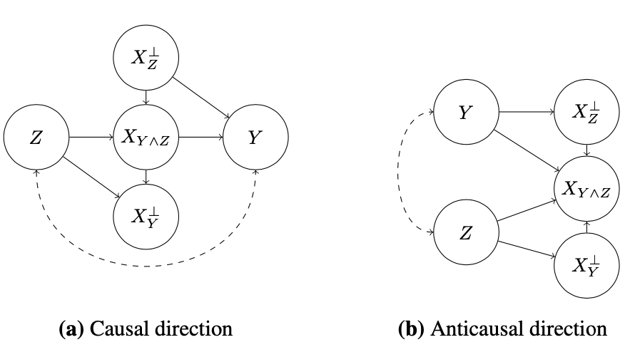
The first one, predicition in the causal direction
Notice that the only thing that’s relevant about these latent variables is their causal relationship with Y and Z. Accordingly, we’ll decompose the observed variable X into parts defined by their causal relationships with Y and Z. We remain agnostic to the semantic interpretation of these parts. Namely, we define $X_{Z}^⊥$ as the part of X that is not causally influenced by Z (but may influence Y ), $X_{Y}^⊥$ as the part that does not causally influence Y (but may be influenced by Z), and $X_{Y∧Z}$ is the remaining part that is both influenced by Z and that influences Y .
Question: why the part $X_{Y∧Z}$ exists? An example was given:
a very enthusiastic reviewer might write a longer, more detailed review, which will in turn be more helpful.
It seems that $Z$ is “being enthusiastic”, $X_{Y∧Z}$ is “being a longer, more detailed review”. Can a stress test be designed w.r.t. such $Z$ ? Why models should be invariant to such $Z$ ? I am a little bit confusing.
The second, predicition in the anti-causal direction
In this graph, the observed X is influenced by both Y and Z. The following example is given:
Example 2.2 We want to predict the star rating Y of movie reviews from the text X. However, we find that predictions are influenced by the movie genre Z.
Question: why in this example, the movie genre Z is not directly influence the star rating Y? What is the $X_{Y∧Z}$ ?
For example, if Adam Sandler tends to appear in good comedy movies but bad movies of other genres then seeing “Sandler” in the text induces a dependency between sentiment and genre.
Question: why “Adam Sandler”, the name of an actor, is in $X_{Y∧Z}$ ?
Second, Z and Y may be associated due to a common cause, or due to selection effects in the data collection protocol—this is represented by the dashed line between Z and Y . For example, fans of romantic comedies may tend to give higher reviews (to all films) than fans of horror movies. Here “fans of some genre” is the confounder.
More explainations on the non-causal associations between Y and Z
First, Y and Z may be confounded: they are both influenced by an unobserved common cause U .
For example, people who review books may be more upbeat than people who review clothing. This leads to positive sentiments and high helpfulness votes for books, creating an association between sentiment and helpfulness.
In this example, “reviewer type” is the confounder.
Second, Y and Z may be subject to selection: there is some condition (event) S that depends on Y and Z, such that a data point from the population is included in the sample only if S = 1 holds.
For example, our training data might only include movies with at least 100 reviews. If only excellent horror movies have so many reviews (but most rom-coms get that many), then this selection would induce an association between genre and score.
Here Y and Z are causes of S.
In addition to the non-causal dashed-line relationship, there is also dependency induced by between Y and Z by $X_{Y ∧Z}$ . Whether or not each of these dependencies is “spurious” is a problem-specific judgement that must be made by each analyst based on their particular use case. However, there is a special case that captures a common intuition for purely spurious association.
Definition 2.3. We say that the association between Y and Z is purely spurious if Y ⊥ X | $X_Z^⊥, Z$ . That is, if the dashed-line association did not exist (removed by conditioning on Z) then the part of X that is not influenced by Z would suffice to estimate Y .
With that language, many existing works focus purely spurious features.
Observable Signatures of Counterfactually Invariant Predictors
How the counterfactually invariant predictors be like? It depends only on $X_Z^⊥$, intuitively. To formalize that idea, we should first show that such a $X_Z^⊥$ is well-defined.
Lemma 3.1. Let $X_Z^⊥$ be a X -measurable random variable such that, for all measurable functions f , we have that f is counterfactually invariant if and only if f(X) is $X_Z^⊥$ -measurable. If Z is discrete then such a $X_Z^⊥$ exists.
Now counterfactually invariant predictors are defined as $X_Z^⊥$-measurable functions.
Theorem 3.2. If f is a counterfactually invariant predictor:
- Under the anti-causal graph, f(X) ⊥ Z | Y .
- Under the causal-direction graph, if Y and Z are not subject to selection (but possibly confounded), f(X) ⊥ Z.
- Under the causal-direction graph, if the association is purely spurious , and Y and Z are not confounded (but possibly selected), f(X) ⊥ Z | Y .
The procedure is then: if the data has causal-direction structure and the Y ↔ Z association is due to confounding, add the marginal regularization term to the the training objective. If the data has anti-causal structure, or the association is due to selection, add the conditional regularization term instead.
A key point is that the regularizer we must use depends on the true causal structure. The conditional and marginal independence conditions are generally incompatible . Enforcing the condition that is mismatched to the true underlying causal structure may fail to encourage counterfactual invariance, or may throw away more information than is required.
How counterfactual invariance relates to OOD accuracy
- First, we must articulate the set of domain shifts to be considered. In our setting, the natural thing is to hold the causal relationships fixed across domains, but to allow the non-causal (“spurious”) dependence between Y and Z to vary. We want to capture spurious domain shifts by considering domain shifts induced by selection or confounding.
- Changes to the marginal distribution of Y will affect the risk of a predictor, even in the absence of any spurious association between Y and Z. Therefore, we restrict to shifts that preserve the marginal distribution of Y .
Definition 4.1. (causally compatible) We say that distributions P, Q are causally compatible if both obey the same causal graph, P(Y ) = Q(Y ), and there is a confounder U and/or selection conditions S, S ̃ such that P=$\int$X,Y,Z | U,S=1)dP ̃(U) and Q=$\int$(X,Y,Z | U,S ̃=1)dQ ̃(U) for some P ̃ ( U ) , Q ̃ ( U ) .
Theorem 4.2. Suppose that the target distribution Q is causally compatible with the training distribution P. Suppose that any of the following conditions hold:
1.the data obeys the anti-causal graph
- the data obeys the causal direction graph, there is no confounding (but possibly selection), and the association is purely spurious, or
- the data obeys the causal-direction graph, there is no selection (but possibly confounding), the association is purely spurious and the causal effect of $X^⊥_Z$on Y is additive.
Then, the training domain counterfactually invariant risk minimizer is also the target domain counterfactually invariant risk minimizer.
Remark 4.3. The causal case with confounding requires an additional assumption (additive structure) because, e.g., an interaction between confounder and $X^⊥_Z$ can yield a case where $X^⊥_Z$ and $Y$ have a different relationship in each domain (whence, out-of-domain learning is impossible).