Your Classifier is Secretly An EBM and You Should Treat It Like One
This is an inspiring work on ICLR 2020 about how to realize the potential of generative models on downstream discriminative problems.
The contributions of this paper:
- They present a novel and intuitive framework for joint modeling of labels and data.
- The new model outperform state-of-the-art hybrid models at both generative and discriminative modeling.
- It is shown that the incorporation of generative modeling gives the model improved calibration, out-of-distribution detection, and adversarial robustness, performing on par with or better than hand-tailored methods for multiple tasks.
As this paper is well written, easy to understand and so far I have little knowledge about EBM , this post just faithfully retells the original paper. It would be good to directly read the paper.
For decades, research work on generative models has been motivated by the promise that generative model can benefit downstream works such as semi-supervised learning, imputation of missing data, and calibration of uncertainty. However, most recent research on deep generative models ignores these problems, and instead focuses on qualitative sample quality and log-likelihood on heldout validation sets.
Currently, a large performance gap exists between the strongest generative modeling approach to downstream tasks and hand-tailored solutions for each specific problems. One potential explanation is that most downstream tasks are discriminative in nature and state-of-the-art generative models are diverged quite heavily from state-of-the-art discriminative architectures. Thus, even when trained solely as classifiers, the performance of generative models is far below that of the best discriminative models. Hence, the potential benefit from the generative component of the model is far outweighed by the decrease in discriminative performance.
This paper advocates the use of energy based models (EBMs) to help realize the potential of generative models on downstream discriminative problems. While EBMs are challenging to work with, they fit more natually within a discriminative framework than other generative models and facilitate the use of modern classifier architectures.
Energy Based Models
Energy based models hinge on the observation that any probability density $p(\mathbf{x})$ for $\mathbf{x} \in \mathbb{R}^D$ can be expressed as
$$ p_\theta(\mathbf{x}) = \frac{\exp(-E_\theta(\mathbf{x}))}{Z(\theta)}, \tag{1} $$
where $E_\theta(\mathbf{x}): \mathbb{R}^D \rightarrow \mathbb{R}$ , known as the energy function, maps each point to a scalar, and $Z(\theta)=\int_{\mathbf{x}} \exp \left(-E_{\theta}(\mathbf{x})\right)$ , is the normalizing constant known as the partition function. In this way one can parametrize an EBM using any function that takes $\mathbf{x}$ as the input and returns a scalar.
For most choices of $E_\theta$, one cannot compute or even reliably estimate $Z(\theta)$, which means standard MLE estimation of the parameters $\theta$ is not straightforward. Thus we must rely on other methods to train EBMs. Note that:
$$ \frac{\partial \log p_{\theta}(\mathbf{x})}{\partial \theta}=\mathbb{E}_{p_{\theta}\left(\mathbf{x}^{\prime}\right)}\left[\frac{\partial E_{\theta}\left(\mathbf{x}^{\prime}\right)}{\partial \theta}\right]-\frac{\partial E_{\theta}(\mathbf{x})}{\partial \theta}, \tag{2} $$
where the expectation is over the model distribution $p_{\theta}(\mathbf{x})$ , which is hard to directly draw samples from. Recent successes of training large-scale EBMs parametrized by deep neural networks have approximated the expectation using a sampler based on Stochastic Gradient Langevin Dynamics(SGLD). It draws samples following $$ \mathbf{x}_{0} \sim p_{0}(\mathbf{x}), \quad \mathbf{x}_{i+1}=\mathbf{x}_{i}-\frac{\alpha}{2} \frac{\partial E_{\theta}\left(\mathbf{x}_{i}\right)}{\partial \mathbf{x}_{i}}+\epsilon, \quad \epsilon \sim \mathcal{N}(0, \alpha) \tag{3} $$ where $p_0(\mathbf{x})$ is typically a uniform distribution over the input domain, and the step-size $\alpha$ decayed following a polynomial schedule.
What Your Classifier is Hiding
Typically, a classification problem with $K$ classes is addressed using a parametric function $f_\theta : \mathbb{R}^D \rightarrow \mathbb{R}^K$ , mapping each data point $\mathbf{x} \in \mathbb{R}^D$ to $K$ real-valued numbers known as logits. These logits $f_\theta(\mathbf{x})$ are used to parametrize a categorical distribution using the so-called Softmax transfer function: $$ p_{\theta}(y \mid \mathbf{x})=\frac{\exp \left(f_{\theta}(\mathbf{x})[y]\right)}{\sum_{y^{\prime}} \exp \left(f_{\theta}(\mathbf{x})\left[y^{\prime}\right]\right)}, \tag{4} $$ where $f_{\theta}(\mathbf{x})[y]$ indicates the $y^{th}$ index of $f_{\theta}(\mathbf{x})$.
In this work, they re-interpret the logits to define $p(\mathbf{x}, y)$ and $p(\mathbf{x})$ as well. They define an energy based model of $p(\mathbf{x}, y)$ via: $$ p_{\theta}(\mathbf{x}, y)=\frac{\exp \left(f_{\theta}(\mathbf{x})[y]\right)}{Z(\theta)}, \tag{5} $$ where $Z(\theta)$ is the unknown normalizing constant and $E_\theta(\mathbf{x}, y) = -f_{\theta}(\mathbf{x})[y]$.
By marginalizing $y$, we obtain $$ p_{\theta}(\mathbf{x})=\sum_{y} p_{\theta}(\mathbf{x}, y)=\frac{\sum_{y} \exp \left(f_{\theta}(\mathbf{x})[y]\right)}{Z(\theta)}, \tag{6} $$ where $E_{\theta}(\mathbf{x})=- \operatorname{LogSumExp}_{y}\left(f_{\theta}(\mathbf{x})[y]\right)=-\log \sum_{y} \exp \left(f_{\theta}(\mathbf{x})[y]\right)$.
Unlike typical classifiers, where shifting the logits by an arbitrary scalar does not affect the model at all, in this framework, shifting the logits for a data point $\mathbf{x}$ will affect $\log p_\theta(\mathbf{x})$. Thus, they makes use of the extra degree of freedom hidden within the logits to define $p(\mathbf{x}, y)$ and $p(\mathbf{x})$ . This approach is refered to as JEM (Joint Energy-based Model).
Optimization
Since maximizing the likelihood of $p_\theta(\mathbf{x}, y)$ and $p_\theta(\mathbf{x})$ is not easy, they propose to use the following factorization: $$ \log p_{\theta}(\mathbf{x}, y)=\log p_{\theta}(\mathbf{x})+\log p_{\theta}(y|\mathbf{x}). $$ $p_{\theta}(y|\mathbf{x})$ is optimized using standard cross-entropy, $p_\theta (\mathbf{x})$ is optimized using Equation $(2)$ with SGLD. They find alternative factoring $\log p(y)+\log p(\mathbf{x}|y)$ lead to considerably worse performance.
Applications
All architectures used are based on Wide Residual Networks. All models were trained in the same way with the same hyper-parameters which were tuned on CIFAR10. Here we introduce two applications of JEM.
Hybrid Modeling
In this part they show that a given classifier architecture can be trained as an EBM to achieve competitive performance as both a classifier and a generative model.
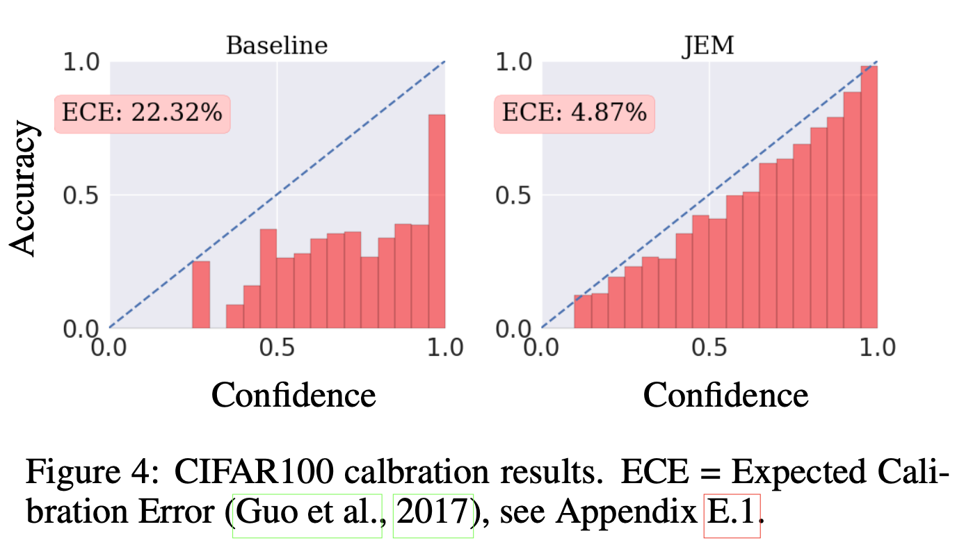
Calibration
A classifier is considered calibrated if its predictive confidence $\max_y p(y|\mathbf{x})$, aligns with its misclassification rate. Thus, when a calibrated classifier predicts label $y$ with confidence .9 it should have a 90% chance of being correct. This is an important feature for a model to have when deployed in real-world scenarios where outputting an incorrect decision can have catastrophic consequences. The classifier’s confidence can be used to decide when to output a prediction or deffer to a human, for example. Here, a well-calibrated, but less accurate classifier can be considerably more useful than a more accurate, but less-calibrated model.
The experiment results on CIFAR100 shows that JEM produces a nearly perfectly calibrated classifier when measured with Expected Calibration Error.